
Serverless Allocation Models For ETL And AI Workloads
If I had to sum this up in one line: I’d match serverless settings to the workload’s tightest limit first - latency for inference, throughput for ETL, warehouse pressure for dbt, and join size plus freshness for feature jobs.
That simple rule avoids a lot of bad setups. A job that scores a checkout event in under 100 ms should not be sized like a batch load that starts at 2:00 AM and processes 1,500 GB. And if I use the same memory, timeout, and concurrency defaults for both, I’m asking for slow responses, extra cost, or failed runs.
Here’s the short version:
- ETL pipelines work best when I size for the heaviest transform, not the average file.
- dbt runs are usually limited more by compile time and warehouse queueing than by local container power.
- Feature engineering jobs often break on large joins, backfills, and burst fan-out.
- Inference endpoints live or die by p95/p99 latency, cold starts, and per-instance memory.
The four knobs that matter most are:
- Memory sizing
- Timeout limits
- Concurrency controls
- Scaling triggers
A few numbers from the article make the split clear:
- Light ETL work often fits in 512–1,024 MB with 30–120 second timeouts.
- AWS Lambda can add up to 1,000 new execution environments every 10 seconds.
- dbt teams often start with 4 threads and then watch warehouse queues before increasing.
- Real-time inference often targets about 50–500 ms p99 for classic ML, and 500–2,000 ms for heavier deep learning.
- Async inference can handle payloads up to about 1 GB and run for up to 15 minutes per request.
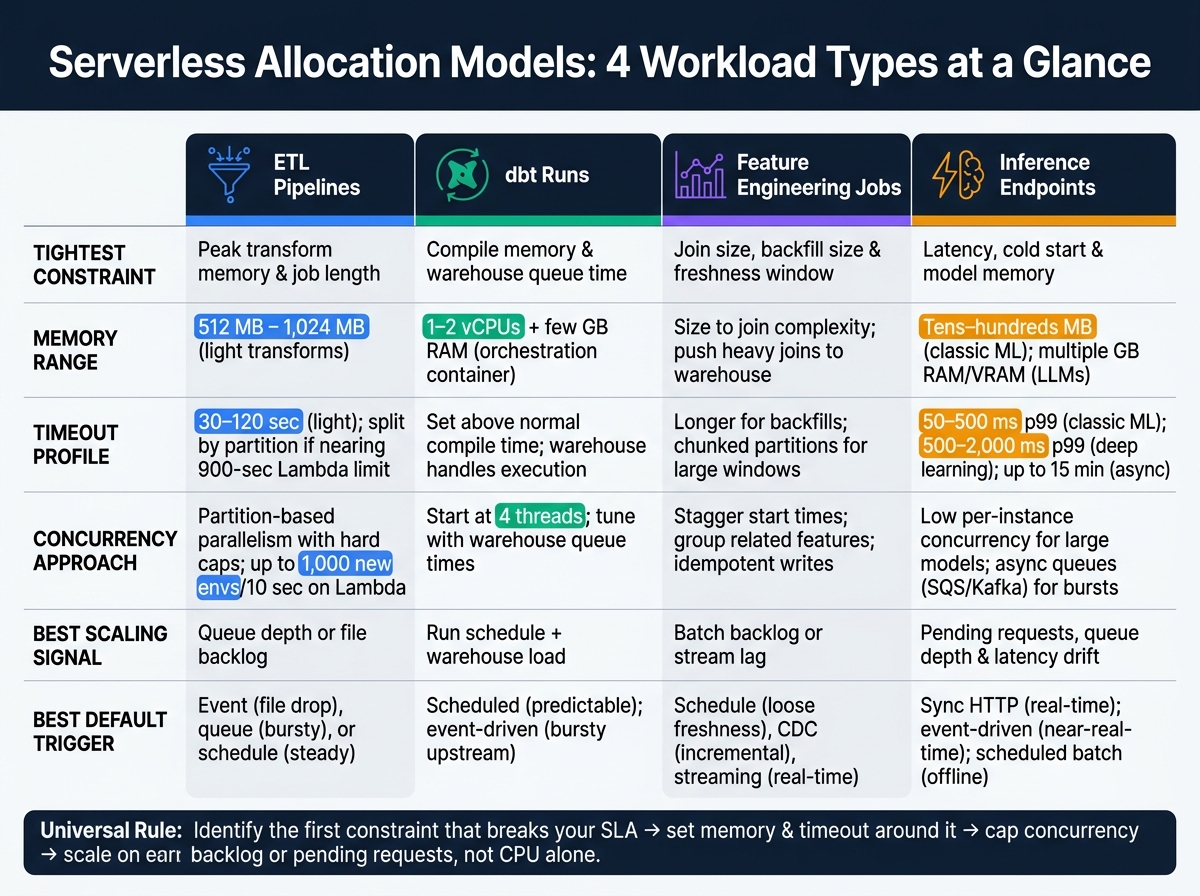
Serverless Allocation Settings by Workload Type: ETL, dbt, Feature Engineering & Inference
Quick Comparison
| Workload | Main limit I’d watch first | Best default trigger | Concurrency approach | Scaling signal |
|---|---|---|---|---|
| ETL pipelines | Peak transform memory and job length | Event, queue, or schedule based on input pattern | Partition-based parallelism with caps | Queue depth or file backlog |
| dbt runs | Compile memory and warehouse queue time | Usually scheduled | Tune --threads with warehouse slots |
Run schedule plus warehouse load |
| Feature engineering jobs | Join size, backfills, freshness window | Schedule, CDC, or streaming | Stagger jobs and control fan-out | Batch backlog or stream lag |
| Inference endpoints | Latency, cold start, model memory | Sync for live traffic; async/batch for slower paths | Low per-instance concurrency for large models | Pending requests, queue depth, latency drift |
So if you want a clean starting point, I’d do this:
- Pick the first constraint that can break the SLA
- Set memory and timeout around that limit
- Put hard caps on concurrency
- Scale on backlog or pending requests, not CPU alone
That’s the core idea behind the full article. The rest is about how those same four settings change across ETL, dbt, feature jobs, and inference serving.
sbb-itb-61a6e59
1. ETL Pipelines
ETL allocation starts with two things: how data shows up and how much arrives at once. An S3 file drop, a nightly 10 TB load, and a queue-based enrichment job do not need the same setup. For ETL work, the trigger you pick shapes how hard you can push memory, timeout, and concurrency.
Trigger Model
Object storage events work well for file drops that need to start right away. Queue triggers are a better fit for bursty upstream systems because they add a buffer and help protect downstream services from getting flooded. Scheduled runs make sense for steady, predictable loads where hour-level freshness is fine.
Once you know the trigger model, size memory around the heaviest step in the pipeline, not the easiest one.
Memory and Timeout Profile
File size can be misleading. A file may look small enough on paper, but parsing, joins, and serialization often drive the highest memory use. So the safer move is to size for peak memory demand, not average usage.
Light transforms often fit within 512–1,024 MB and a 30–120 second timeout. Larger files or CPU-heavy work, like wide joins or deduplication, usually need more room and more time. And if a job starts pushing against the 900-second Lambda limit, don't just keep stretching the timeout. Split the work by partition or time window instead.
Concurrency Pattern
Running one file per invocation is simple. It also starts to crack when volume climbs and orchestration overhead becomes a bigger problem than the compute itself.
A better pattern is partition parallelism. Split work by date, tenant, or region so separate jobs can run side by side without colliding. This is where bounded worker pools help too, especially when downstream systems have connection limits or rate caps.
AWS Lambda can scale a single function by 1,000 concurrent execution environments every 10 seconds. That sounds great until uncapped fan-out starts hammering databases and object stores.
Scaling Strategy
For bursty ETL, queue depth is usually the clearest scaling signal. Event triggers are still a good fit when you need lower-latency file handling. Either way, add concurrency caps, retries, and dead-letter queues so failures don't spiral into extra cost or backpressure problems.
Those same knobs shift in dbt runs, where compilation time and warehouse calls change the allocation profile.
2. dbt Runs

dbt runs use a short-lived container to compile models and send SQL to the warehouse. The warehouse handles the heavy lifting. So the main allocation shift moves away from local compute and toward orchestration overhead and warehouse capacity.
You’ll usually notice that shift in a pretty clear order: first in triggers, then compile memory, then concurrency, and finally warehouse scaling.
Trigger Model
Use schedules when run timing is predictable. Use event-driven triggers when upstream data arrives at uneven times and your setup needs to handle bursts.
Schedules tend to lower allocation risk. Event-driven runs tend to increase it.
Once you’ve picked the trigger, the next limit usually isn’t event ingestion. It’s compile-time memory.
Memory and Timeout Profile
Plan for two phases: compile and run.
Compilation can put pressure on memory in large projects. Execution, on the other hand, shifts most of the load to the warehouse. That’s an important distinction, because people often size the container for the run itself when the bigger issue is the compile step.
In most cases, the orchestration container needs only 1–2 vCPUs and a few GB of RAM. Compile timeouts should sit a bit above normal compile times. Size the warehouse for the run window, not the container.
A dbt Labs case study reported that optimizing 26 models cut runtime 45% and saved about $22,000 a year, even after moving to a larger warehouse.
Concurrency Pattern
dbt manages in-job parallelism with the --threads setting. That setting controls warehouse connections, not local CPU threads.
Start small. The dbt community points to 4 threads as a baseline for BigQuery, then increase only after watching warehouse queue times.
--threads and run slots need to be tuned together. More threads can still make runs slower if warehouse queueing starts to climb. It’s a bit like opening more checkout lanes in a store when the stockroom is already jammed - on paper it sounds faster, but the bottleneck just moves.
After concurrency is dialed in, the next step is matching warehouse size to the run pattern.
Scaling Strategy
For nightly full refreshes, scale the warehouse up. For frequent incremental models, keep runs smaller and tighter.
The best cost control for dbt is usually auto-suspend and auto-resume on the warehouse. Teams pay for active query time, not 24/7 uptime. Pair that with incremental models and partitioning or clustering so scan sizes stay under control as data grows.
There’s also a tipping point to watch for. When runtime gets close to the trigger interval, the warehouse is basically always on. At that point, the cost model stops acting like serverless.
3. Feature Engineering Jobs
Unlike dbt, feature jobs usually handle their own joins and aggregations before writing to offline and online stores. That means the compute load doesn't move neatly into the warehouse, and that changes how you size and assign resources.
Trigger Model
Scheduled refreshes work well for features with loose freshness needs, like daily or weekly engagement scores or customer lifetime value. In those cases, downstream models can handle data that's a few hours old.
Event-driven jobs are a different story. They use streaming systems like Kafka or Spark Structured Streaming for features where stale data can break fraud checks, recommendation systems, and bidding decisions.
CDC-based incremental runs sit in the middle. They process only new or changed data on a short cadence, which gives you lower lag without the overhead of a full streaming pipeline. Backfills need more room to breathe: larger batch windows, longer runtimes, and chunked partitions.
Memory and Timeout Profile
Join-heavy feature jobs are where serverless memory limits start to hurt. Picture a pipeline joining customer records, support events, authentication logs, orders, and marketing data across tens of millions of rows. It doesn't take much for that to outgrow a function's memory.
A better setup is to push heavy joins into the warehouse or lakehouse and keep serverless focused on orchestration and I/O. One common pattern is to pre-aggregate at the entity level first, then join the smaller tables in a second stage.
Concurrency Pattern
Scheduled batch refreshes tend to create burst concurrency. A lot of feature tasks kick off at the same time and hammer the same warehouse, object storage, and feature store all at once. That's how you end up with throttling or connection pool exhaustion.
You can soften that spike by:
- Staggering start times
- Grouping related features into fewer, larger jobs
Event-driven jobs behave more like traffic on a highway: volume goes up at peak times and drops when activity slows. Because of that, idempotent writes matter. Retries shouldn't corrupt feature values, and backpressure controls help keep the online store from getting flooded.
After trigger choice and concurrency, allocation usually splits into offline batch jobs and online serving paths.
Scaling Strategy
Feature scaling splits into offline batch and online serving.
Offline jobs scale with distributed batch engines, time-based partitioning, and elastic cloud storage, sized to finish within the freshness SLA. Online serving paths scale horizontally through key-based sharding and stateless ingestion microservices, with the store partitioned by entity ID hash to isolate hot keys.
Training data also needs to be point-in-time correct. That means point-in-time joins must use only values that were known at the event time. Skip that step, and you get data leakage. The worst part? It can quietly drag down model performance and lead to costly re-runs.
When features move to real-time serving, the allocation model shifts again.
4. Inference Endpoints
Inference endpoints are a different beast because the shape of the request changes almost everything: latency, memory use, and how the system scales. A fraud check at checkout and a nightly batch re-ranking job both run models, but they don’t need the same setup at all. That’s why the first allocation call is usually the trigger model. After that, you size memory, concurrency, and scale around it.
Trigger Model
Synchronous HTTP triggers are the default for real-time inference, like chat completions or fraud checks at checkout. The caller waits for the answer, so latency matters right away. In many cases, p99 targets land around 50–500 ms for classic ML models and 500–2,000 ms for heavier deep learning models.
Event-driven triggers fit near-real-time work, like fraud scoring on transaction streams. Requests land in a queue, and workers process them on their own pace instead of matching the incoming rate second by second. Scheduled batch triggers are built for nightly or hourly scoring jobs, where throughput and cost matter more than response time.
Managed services usually expose these same three patterns: real-time, async, and batch.
Memory and Timeout Profile
Once the trigger is set, the next hard limit is usually model size and cold-start cost. Small gradient-boosted tree or logistic regression models may fit in tens to hundreds of megabytes, which keeps cold starts shorter and makes memory duplication across replicas less painful.
Transformer-based models and LLMs are a different story. Each replica may need its own full copy of the weights, and that can mean multiple gigabytes of RAM or GPU VRAM. At that point, memory isn’t some side detail. It often becomes the main constraint.
A common setup is a two-tier architecture: a thin serverless API layer handles auth, validation, and routing, then forwards requests to a warm model-serving tier that keeps model weights loaded and keeps connections to feature stores or vector databases warm. That split helps avoid paying the cold-start penalty on the heavy part of the stack for every request.
Asynchronous endpoints also stretch much farther on job size. They support payloads up to about 1 GB and processing times up to 15 minutes per request. That makes them a better match for heavy multimodal or video generation work than synchronous functions.
Concurrency Pattern
Concurrency gets expensive fast because every concurrent execution generally loads its own copy of the model into memory. With large models, that means the first wall you hit during a traffic spike is often memory or cost, not CPU.
For synchronous endpoints, that usually means keeping per-instance concurrency limits conservative and shedding load when traffic jumps. There’s no magic here. If too many requests hit a large model at once, the system can run out of room fast.
Async pipelines handle bursts in a much calmer way. Durable queues like SQS or Kafka absorb the spike, and workers drain jobs at a steady rate that matches available capacity. That decouples incoming traffic from execution speed, which is exactly what you want when load arrives in waves.
The failure mode also changes by trigger type:
- Synchronous throttling returns HTTP 429 errors to callers
- Asynchronous invocations are queued and retried automatically
Scaling Strategy
The tradeoff between scale-to-zero and provisioned capacity mostly comes down to latency tolerance and traffic shape.
Scale-to-zero works well for spiky, low-volume workloads with small models and no tight latency SLA. The upside is simple: idle cost drops to $0. The downside is cold starts, which can add hundreds of milliseconds or more.
For customer-facing endpoints with strict p95 or p99 targets, provisioned concurrency is often the safer call. It pre-initializes a fixed number of environments, so requests skip cold start entirely, but you pay for idle capacity. That trade can feel annoying on paper, but if the endpoint sits on a checkout flow or user-facing product path, the math usually changes fast.
A practical middle ground is to set a provisioned floor around expected baseline traffic, then let auto-scaling add replicas when a real spike hits. That gives you a steady base without keeping the whole fleet hot all day for no reason.
GPU-based endpoints add one more wrinkle. GPU nodes cost a lot and take time to spin up, so teams usually keep a warm pool and rely on batching to keep utilization high enough to justify the spend.
Use the serving model that fits the latency budget: synchronous for sub-second p99 targets, with provisioned capacity for customer-facing paths; async queues for workloads that can wait seconds to minutes; and batch transforms for offline scoring where job-level throughput is the only thing that matters.
Tradeoffs and Pros and Cons by Workload
These workload-specific settings boil down to a few practical defaults. There’s no one-size-fits-all serverless allocation model. The right setup depends on the shape of the work: unpredictable ETL and feature backfills do well with elastic triggers, dbt fits scheduled runs, and inference needs protected low-latency capacity.
Use this comparison to pick a default allocation pattern before you start tuning edge cases. The table below condenses the main tradeoffs across four levers that matter most: memory, timeout, concurrency, and scaling trigger.
| ETL Pipelines | dbt Runs | Feature Engineering Jobs | Inference Endpoints | |
|---|---|---|---|---|
| Strengths | Scales with bursty, irregular data; can scale to zero when idle | Parallelizes models and tests; fits dependency graphs and scheduled runs | Absorbs backfills and retraining spikes; strong horizontal burst tolerance | Automatic horizontal scaling under variable request load |
| Weaknesses | Cold starts delay time-sensitive loads; long jobs may hit execution time limits | Less flexible for ad hoc runs; heavy DAGs can exceed memory or timeout thresholds | Repeated cold starts hurt throughput; large scans can overwhelm feature stores | Tail latency spikes during cold starts; memory caps constrain large models |
| Cost risk | Low at idle; higher when large bursts repeat often or triggers are misconfigured | Moderate from scheduled warehouse usage and frequent CI runs | Medium if backfills are large and uncontrolled | High if autoscaling is uncapped or provisioned capacity is sized for peak traffic all day |
| Operational risk | Medium - retries, timeouts, and state handling need explicit design | Low to medium when schedules and timeouts are well managed | Medium if scaling lags or tasks fan out too aggressively | High for user-facing paths - latency misses are visible to end users immediately |
| Safest default config | Conservative timeout, idempotent retries, scheduled execution for critical loads | Scheduled job on a warehouse with explicit size control and defined timeout | Controlled concurrency, defined timeout, downstream backpressure | At least one warm replica or provisioned concurrency; scale-to-zero only for low-volume or non-critical traffic |
The pattern is pretty straightforward. ETL and feature backfills usually do best with elastic batch scaling. dbt is a better fit for scheduled orchestration. Feature prep needs autoscaling that can handle bursts without letting fan-out get out of hand. Inference is different again: it needs guarded low-latency capacity, because users feel delays right away.
For bursty workloads, scale on queue depth or pending requests, not CPU alone. CPU can miss the early warning signs. Backlog and request buildup tell you sooner when latency is about to drift.
Conclusion
Serverless allocation depends on the workload. It’s not a one-size-fits-all setup. The shape of the workload should drive the config, and ETL pipelines, dbt runs, feature engineering jobs, and inference endpoints all behave differently.
Across these four workload types, the best default usually comes from the tightest constraint. Here’s a fast way to pick a starting point:
| Priority | Dimension | Workload Type | Starting Config |
|---|---|---|---|
| 1 | Latency target (<200–300 ms) | Inference endpoints | Low per-instance concurrency, generous memory, warm pools or provisioned concurrency for large models |
| 2 | Freshness SLA (every 5–15 min) | Near-real-time ETL and feature jobs | Moderate to high memory, moderate timeouts, queue-depth scaling |
| 3 | Data volume (high, relaxed SLA) | Batch ETL | Higher memory, longer timeouts, scheduled scaling |
| 4 | Request burstiness | All types | Fast scale-out for high burstiness; slower scaling for steady traffic |
A simple rule works well here: start with the first constraint that actually binds. Then tweak the rest only if a bottleneck still shows up.
It also helps to put one guardrail in place from day one: define a profile for each workload class - Batch-ETL, Scheduled-dbt, Feature-Online, Inference-Interactive - with target SLAs and default ranges for all four levers. Turning those profiles into configuration templates in Terraform, CloudFormation, or internal tooling cuts down on ad hoc misconfigurations and makes changes much easier to review before they hit production.
For hands-on practice, DataExpert.io Academy offers boot camps and labs for ETL, feature, and inference pipelines on AWS, Databricks, and Snowflake.
FAQs
How do I choose the right serverless profile for my workload?
Choose serverless for ad hoc, bursty, or hard-to-predict workloads. It scales on its own, and you don’t pay for idle capacity sitting around. If demand is steady and you want more control, use job compute or job clusters for scheduled ETL.
For sizing, match resources to the shape of the workload. Complex transformations usually need more memory. Wide transformations often run better on fewer, larger nodes. And irregular inference or feature workloads do well with instant scaling when concurrency spikes hit.
When should I scale on queue depth instead of CPU?
Scale based on queue depth when the bottleneck is concurrency, not raw compute power. If tasks keep sitting in the queue or remain scheduled even though resources look available, that usually means the system has hit its limit for handling many requests at the same time.
In that situation, scale out by adding more workers or clusters.
Increase CPU and memory only when the work itself is slow because of heavy computation, memory spillage, or high I/O.
What’s the biggest mistake when sizing memory and concurrency?
The biggest mistake is mixing up memory and concurrency. That mix-up usually leads to the wrong scaling move.
If performance is limited by memory, scaling out gives you more concurrency, but it doesn't solve the memory problem. On the flip side, if the slowdown comes from queue time, just making the warehouse bigger is often a poor use of spend.
There's another issue to watch closely: disk spill. When memory runs low, data can move from local SSDs to slower remote storage. That switch can hurt performance by up to 10x.
So before changing anything, check two things:
- Memory use
- Queuing time
That makes it much easier to match the fix to the actual bottleneck, instead of throwing more compute at the wrong problem.